


By Brent A Gregory and Oleg Moroz, Creative Power Solutions (CPS)
In a modern gas turbine, up to about 20% of the main compressor (inlet) flow is bled off to perform cooling and sealing of hot-section components. Cooling flows are necessary for the engine to function. However, too much cooling has a negative impact on performance and output. To optimize performance, one must know what cooling flows to monitor and control.
Using a four-stage turbine as an illustration, here’s how critical components are cooled (in order of decreasing flow):
- Vane 1. Cooling to first-stage turbine vanes is provided internally to keep materials at a safe temperature.
- Rotor and blade cooling. An external pipe takes air from the engine’s compressor, cools it in an external heat exchanger, and directs the cool air to turbine blades and the rotor.
- Vane 2. Two pipes (a main line and a bypass) provide cooling air to second-stage vanes.
- Vane 3. Two pipes (a main line and a bypass) provide cooling air to third-stage vanes.
- Vane 4. Two pipes (a main line and a bypass) provide cooling air to fourth-stage vanes.
Some OEMs rely on coolant delivery systems other than pipes. Example: They may channel cooling flow through the major internal skeletal structure of the engine.
Important to this discussion is that Vane 1 and rotor and blade cooling flows usually cannot be adjusted because they are determined by engine design. When an external pipe delivers cooling air to the turbine rotor and its blades, that flow can be monitored easily. While Vane 1 cooling flow generally is not measured, a thermocouple in the region of the vane “box” helps determine flow using an algorithmic model.
Easiest to measure and control are cooling-air flows to Vanes 2 through 4. The main line carries most of the flow, which is determined by the differences in pressure between the compressor (where the air is extracted) and the turbine (where the cooling air is introduced). Flow is controlled by an orifice in the pipe. The larger the orifice throat area, the more air will pass.
The bypass line, smaller than the main line, has a valve to modulate cooling flow as required by different engine operating conditions. The adjustment is made by the engine control system. Cooling flows for Vanes 2, 3, and 4 are controlled by disc-cavity temperatures. If more cooling flow is need to reduce disc-cavity temperature to the control limit, the valve admits more cooling air. Disc-cavity limits are used to keep turbine parts at a safe operating temperature.
If an engine is having trouble staying within disc-cavity temperature limits, cooling flows can be adjusted by changing orifice plates in the main and/or bypass lines. However, this should be done carefully because changing cooling flows will impact engine life and performance.
One way to monitor cooling flows is to track disc-cavity temperatures and the position of bypass valves. By comparing actual disc-cavity temperatures to control specified temperatures it can be determined if an engine is being overcooled or undercooled.
Another useful exercise is to look at bypass-valve positions for Vanes 2, 3, and 4. If a bypass valve is fully open, it means there’s insufficient cooling flow; if fully closed, the engine is being overcooled. Note that some control systems treat 100% as fully open, others fully closed. Check the appropriate manual to learn how your control system is configured.
Trend both the positions of bypass valves and disc-cavity temperatures over a range of ambient temperatures and engine loads to determine if orifice plates in the main lines and bypass lines are sized properly.
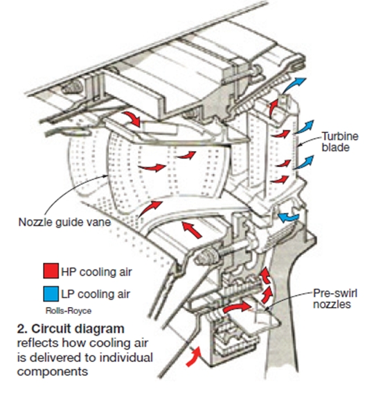
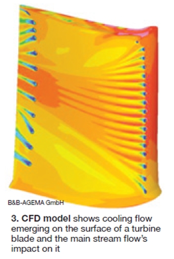
Cooling principles. OEMs may identify engine cooling flows in a diagram often referred to as a worm chart (Fig 1). The numbers in the figure are percentages of total compressor inlet air flow. Cooling flows delivered to individual components are illustrated in Fig 2 for a first-stage vane. Actual representation of cooling flows can be modeled using a sophisticated 3-D characterization of the flow as shown in Fig 3.
Effect of cooling on performance. To demonstrate the effect of cooling flow on the performance of a gas turbine typically used in simple- or combined-cycle service, the authors produced a theoretical model in a commercially available code (GasTurb) and varied cooling flows to see their impacts on the operating point. GasTurb allows engineers to change both the amount of the cooling flow and its energy content.
Click thumbnails to enlarge figures.
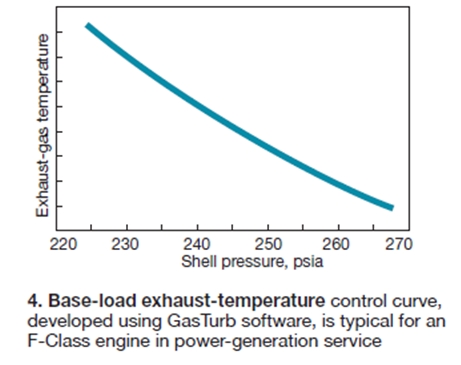
Engine operation overview. At base load, most GTs are operated on an exhaust-temperature control curve (Fig 4) typically created by running the engine model through a range of ambient temperatures at a given design firing temperature. Based on model output and site-specific conditions, a control curve for base-load operation is created.As discussed above, the main purpose of cooling air is to maintain safe vane and blade metal temperatures during gas-turbine operation. Cooling flows have a net positive result on gas-turbine performance. Because cooling air does not go through the combustor, some of the work is lost; however, cooling air permits operation at a higher firing temperature which leads to a higher net power output and better efficiency.
The main disadvantage of the curve is that there’s no awareness of the engine’s actual firing temperature during operation. So, if cooling flow increases, firing temperature increases as well, to maintain the same exhaust temperature for a given shell pressure. Here, firing temperature is defined as the temperature of the gas leaving the combustor—so-called T4.
On the other hand, if the cooling flow decreases, the exhaust temperature increases; this causes a reduction in firing temperature to maintain the exhaust temperature defined by the control curve.
Site-specific GT models are required to predict engine cooling flows. Developing such models usually requires performance software and a significant amount of reliable engine data. Measuring cooling flows is not as complicated. By recording temperature, pressure, and pressure drop across a known orifice, they can be calculated to verify cooling-flow measurements.
One of the primary reasons for tracking cooling flows is to determine how T4 changes with time. Knowing the exact value is not the goal here. With engine variations and the inability to monitor Vane 1 cooling flow, the actual T4 value is difficult to determine. However, knowing how T4 is trending helps you assess engine performance and make appropriate O&M decisions.
Recall the First Law of Thermodynamics from academic study: Energy is always conserved. Simply put, Energy in=Energy out. T4 can be estimated by creating a heat balance around the combustor. First perform a heat balance around the engine to determine total air flow into the GT, then subtract cooling-air flows to calculate the amount of air entering the combustor. Keep in mind that good data are needed for repeatable and valid performance assessments, and this requires that you install proper plant instrumentation and calibrate it regularly.
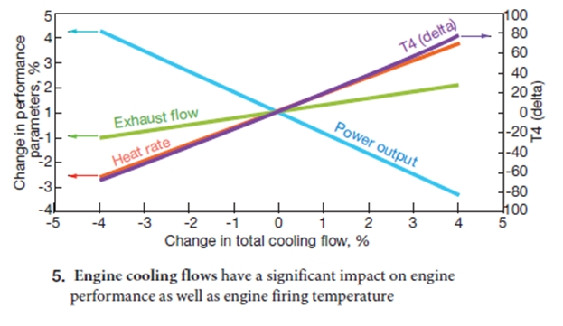
Effect of cooling flows on engine operation. The benefit of monitoring engine cooling flows is better assessment of engine performance and operation. Fig 5 was created using the commercial GasTurb software referenced earlier. An F-Class engine was modeled based on data publicly available. GasTurb uses generic compressor and turbine maps available in the public domain.
The plotted data illustrate the impact of changes in the total engine cooling flow from +4% to -4% on firing temperature, power output, heat rate, and exhaust energy. As mentioned earlier, cooling flows can account for up to about 20% of total engine air flow. The curves were created by keeping the engine on the base-load exhaust-temperature control curve generated by GasTurb and reflect what you would expect to see during operation.
The power and heat-rate impacts are significant from a performance point of view; but just as significant is the impact that firing temperature may have on the lifecycle of turbine parts. Based on experience, increasing the firing temperature by 40 deg F may decrease the life of hot-section parts by as much as 50%. If firing temperature is trended, any spikes or falls in T4 can be identified and investigated immediately. This minimizes the opportunity for surprises that could contribute to unplanned outages or to extensions of planned outages.
Maintaining optimal performance. Another benefit of tracking cooling flows and trending T4: Maintain optimal engine performance and output. As mentioned earlier, the base-load exhaust-temperature control curve is created based on design firing temperature. The control curve is not aware of what the actual engine firing temperature is during operation.
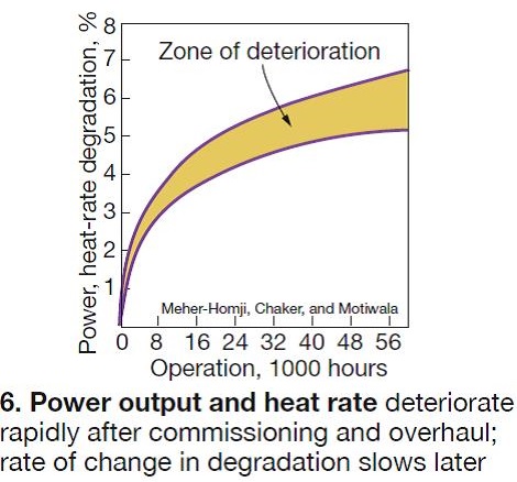
Turbine degradation has an inverse exponential profile. Most of the degradation occurs in the first few thousand hours, with wear and tear leveling out as time goes on. A sample degradation curve is presented in Fig 6. An engine completing an outage may have tight blade clearances in the turbine section as well as new components, such as seals. Clearances will open up as the engine goes through several thermal cycles. Seals also will see most degradation during the first few thousand hours of operation.
After the break-in period, the engine is not able to extract as much energy out of the working fluid, causing the exhaust temperature to rise. The control curve “sees” the exhaust temperature increasing and engine controls respond by reducing firing temperature. While parts lives are extended at the lower firing temperature, engine performance suffers.
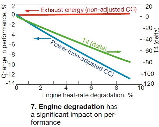
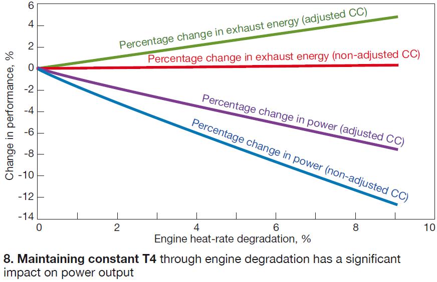
The plot in Fig 8 reflects how engine performance can be optimized by adjusting the base-load control curve, so the engine operates at constant T4. The blue and red curves are the same as in Fig 7. The purple and green curves were developed by keeping the firing temperature at the design level as the engine degrades.Fig 7 illustrates how a decrease in firing temperature caused by engine degradation adversely impacts performance. This chart was developed by holding the GasTurb model on the design exhaust-temperature control curve. Thus T4 is dropping as engine heat rate increases. Note that the heat-rate increase is based on turbine degradation only; compressor degradation is not included. To reiterate, because the turbine is not able to extract as much work out of the working fluid, the exhaust temperature increases and T4 must drop to stay on the control curve.
In Fig 8, the purple curve represents the unrecoverable and expected engine degradation. The blue line reflects the power loss attributed to both the unrecoverable engine degradation and the inability of the control curve to self-adjust and maintain a constant T4 value.
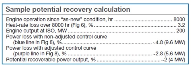 The bottom-line benefit of monitoring cooling flows and trending firing temperature is that when firing temperature drops, the control curve can be adjusted and some of the lost performance and capacity generally can be restored. The table offers an example, based on the the GasTurb model, of the potential power recovery that a control-curve adjustment can achieve. In this case, 4 MW can be restored 8000 hours after commissioning or following an overhaul. But, once again, remember this assumes heat-rate deterioration is due only to turbine degradation mechanism. If compressor degradation were included, the recovery would be less.
Wrap up. Cooling-flow monitoring, together with properly calibrated plant instrumentation, allows for trending of engine firing temperature and performance using fundamental thermodynamics. Due to this monitoring, performance issues arising during engine operation can be accurately assessed and corrections executed during scheduled outages.
A quick way to determine if an engine has cooling issues is to trend disc-cavity temperature and bypass-valve positions for a range of ambient conditions and loads. Bypass valves that are fully open or closed are conducive to engine undercooling or overcooling. Low disc-cavity temperatures are indicative of overcooling; high temperatures mean insufficient cooling.
Neglecting to monitor cooling flows and engine health may lead to an under-performing engine, unnecessary forced outages, or premature replacement of engine components. CCJ